Read Multiple Variables Create New Variable if Not Blank Spss
ane. Introduction
This module will explore missing data in SPSS, focusing on numeric missing information. We will depict how to betoken missing data in your raw data files, how missing data are handled in SPSS procedures, and how to handle missing data in a SPSS information transformations. At that place are two types of missing values in SPSS: i) system-missing values, and 2) user-defined missing values. Nosotros volition demonstrate reading data containing each kind of missing value. Both information sets are identical except for the coding of the missing values. For both information sets, suppose we did a reaction time written report with 6 subjects, and the subjects reaction time was measured 3 times.
2. System-missing values
System-missing
values are values automatically recognized as missing past SPSS. You might notice that some of the reaction times are left bare in the information below. That is the accepted way of indicating system missing data in the data prepare. For example, for subject 2, the second trial is blank. The only way to read raw data with fields left blank is with stock-still field input. The values left bare automatically are treated every bit arrangement-missing values.
Note:
It is possible to hold the missing place with a single dot in the field, merely if you exercise you will get a warning message each time SPSS encounters one of these values. The resulting variable is coded with organisation-missing values.
DATA Listing Fixed/ id 1 trial1 3-5 (1) trial2 6-8 (1) trial3 11-13 (1). Brainstorm DATA . 1 1.5 1.4 1.six 2 1.5 1.9 3 2.0 1.6 4 ii.2 5 two.1 2.3 two.2 6 1.viii 2.0 ane.nine END Information . LIST .
Ane reason for missing data might exist that the equipment failed for that trial was missing. The result of the list follows, notice that SPSS marks system-missing values with a dot in the listing. There is a dot everywhere in the list that at that place was a blank in the information.
ID TRIAL1 TRIAL2 TRIAL3 ane i.5 1.0 ane.6 ii ane.v . one.9 3 . 2.0 1.6 4 . . two.2 five 2.1 ii.0 2.ii 6 1.eight ii.0 1.ix Number of cases read: half dozen Number of cases listed:
three. User-divers missing values
User-divers
missing
values are numeric values that demand to be defined as missing for SPSS. You might notice that some of the reaction times are -9 in the data below. You may use any value you choose to correspond a missing value, but exist conscientious that you lot don't cull a value for missing that already exists for the variable in the data fix. For that reason many people choose negative numbers or large numbers to represent missing values. For example, for subject 2, the second trial is -nine. You may read raw data with user-missing values either equally fixed field input or as costless field input. Nosotros volition read it as complimentary field input in this instance. When defined as such on a missing values control these values of -nine are treated every bit user-missing values.
Data LIST FREE/ id trial1 trial2 trial3 . MISSING VALUES trial1 TO trial3 (-9). COMPUTE trialr1=trial1. COMPUTE trialr2=trial2. COMPUTE trialr3=trial3. VARIABLE LABELS trial1 "Trial ane User Miss" trialr1 "Trial one Sys Miss". BEGIN Information . i 1.5 1.four 1.half dozen 2 1.5 -9 1.nine three -nine 2.0 1.half-dozen 4 -9 -9 two.2 5 2.one 2.3 2.2 half dozen 1.viii ii.0 ane.9 END Data . List .
The compute control is used to create the new variables trialr1 through trialr3, which will incorporate arrangement-missing values where there were user-defined missing values in the original variables. User-defined missing values on the original variable become organisation-missing values on the new variables. The result of the listing follows, notice that SPSS marks user-missing values with a -nine in the listing. In that location is a -9 everywhere in the list that at that place was a -ix in the data, and so the value of the user-defined missing is preserved for the original variables ().
ID TRIAL1 TRIAL2 TRIAL3 TRIALR1 TRIALR2 TRIALR3 ane.00 1.fifty i.twoscore 1.60 1.l 1.40 ane.60 2.00 1.50 -9.00 1.90 1.l . ane.xc 3.00 -ix.00 2.00 1.60 . 2.00 ane.60 4.00 -9.00 -nine.00 2.20 . . 2.20 5.00 2.10 2.30 ii.xx two.x 2.thirty 2.20 6.00 i.80 2.00 i.90 i.80 2.00 one.xc Number of cases read: half-dozen Number of cases listed: half-dozen
Let's examine how SPSS handles missing data in assay commands.
4. How SPSS handles missing data in analysis commands
As a full general dominion, SPSS assay commands that perform computations handle missing data by omitting the missing values. (We say assay commands to bespeak that we are non addressing commands like sort.) The mode that missing values are eliminated is non always the aforementioned among SPSS commands, so allow's us look at some examples. Offset, use the descriptives command on our data file and run across how this control handles the missing values.
DESC /VAR= trial1 trial2 trial3 trialr1 trialr2 trialr3.
Equally you see in the output beneath, descriptives computed the ways using four observations for trial1 and trial2 and six observations for trial3. In short, descriptives used all of the valid data and performed the computations on all of the bachelor data. This was also truthful for the adjacent 3 variables containing user-missing values.
As you run across below, frequencies too performed its computations using just the available data. Note that the percentages are computed based on merely the total number of non-missing cases. But the missing values practice announced in the tables and they are marked equally missing. This is true for both types of missing values.
FREQ /VAR= trial1 trialr1 .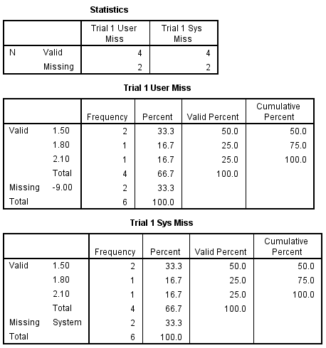
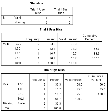
It is possible that you might want the valid percentages to exist computed on the total number of values, and even written report the pct missing in the table itself. Y'all can asking this using the missing=include subcommand on the freq command. This is shown beneath for trial1 and trialr1.
FREQ /VAR= trial1 trialr1 /MISSING= INCLUDE.
As you lot see, now the valid percentages are computed out of the total number of observations, and the per centum missing are shown right in the table as well for the variable trial1 which contained user-missing values. For trialr1, the organisation-missing values are non used to compute percents even with missing=include specified.
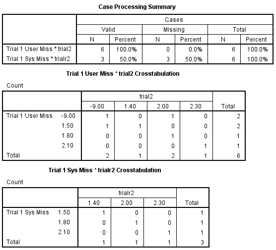
The crosstabs command but includes valid (not-missing data) in its tables. Cases containing a missing value for even i of the variables are not included in the table. Annotation that the percentages are computed based on just the non-missing cases. This is true for both types of missing values.
CROSS /TAB= trial1 By trial2 / trialr1 BY trialr2.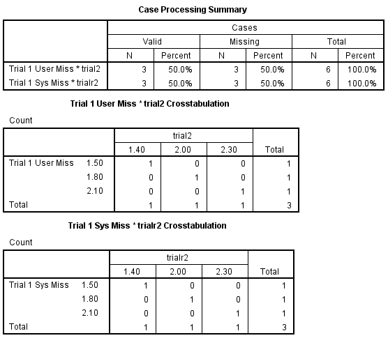
Information technology is possible that yous might desire the missing values included in the tables. This is especially true when you are using crosstabs to verify your transformations. You lot can request this using the missing=include subcommand on the crosstabs command. This is shown below for trial1 and trialr1. Here again, yous will but exist successful for user-missing values.
Cantankerous /TAB= trial1 Past trial2 / trialr1 BY trialr2 /MISSING= INCLUDE.
The user-missing values are included in the tabular array for the variable trial1. For trialr1, the system-missing values are not included in the table even with missing=include specified. There is no subcommand that will enable the inclusion of system-missing values in the crosstabs table.
There is no manner to get a system missing value to announced in a crosstabs table. The closest you lot will come is to change the system-missing value to a user-missing value. This can exist accomplished with a recode command, as is shown below. The keyword sysmis can exist used on the recode command, and it stands for the system-missing value.
RECODE trialr1 trialr2 (SYSMIS=-1) (ELSE=COPY) INTO trialb1 trialb2 . MISSING VALUES trialb1 trialb2 (-1). CROSS /TAB= trialb1 BY trialb2 /MISSING= INCLUDE.
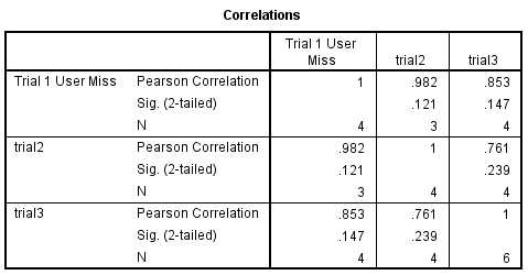
Allow'due south look at how corr handles missing information. We would expect that it would do the computations based on the available data, and omit the missing values for each pair of variables. Considering 2 variables are necessary to compute each correlation. Here is an instance programme.
CORR VAR trial1 trial2 trial3 .
The output of this command is shown beneath. Note how the missing values were excluded. For each pair of variables, corr used the number of pairs that had valid information. For the pair formed by trial1 and trial2, there were three pairs with valid data. For the pairing of trial1 and trial3 there were four valid pairs, and likewise there were four valid pairs for trial2 and trial3. Since this used all of the valid pairs of information, this is oftentimes chosen pairwise deletion of missing data.
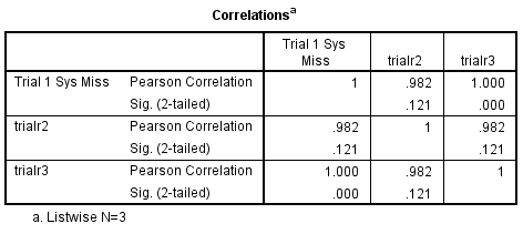
It is possible to specify that the correlations run only on observations that had complete data for all of the variables listed on the var subcommand. You might want the correlations of the reaction times only for the observations that had not-missing data on all of the trials. This is called listwise deletion of missing information meaning that when any of the variables are missing, the entire observation is omitted from the analysis. You can asking listwise deletion within corr with the mssing=listwise subcommand, every bit shown in the example below.
CORR /VAR= trialr1 trialr2 trialr3 /MISSING=LISTWISE.
As y'all come across in the results below, the N for all the simple statistics is the same, 3, which corresponds to the number of cases with consummate non-missing data for trial1, trial2 and trial3. Since the N is the same for all of the correlations (i.e., 3), the Northward is not displayed forth with the correlations in SPSS 7.5 and higher.
5. Summary of how missing values are handled in SPSS assay commands
It is important to understand how SPSS commands used to analyze data treat missing data. To know how any i command handles missing data, y'all should consult the SPSS transmission. Here is a brief overview of how some common SPSS procedures handle missing data.
- DESCRIPTIVES
For each variable, the number of non-missing values are used. You can specify the missing=listwise subcommand to exclude data if there is a missing value on whatever variable in the list.- FREQUENCIES
By default, missing values are excluded and percentages are based on the number of non-missing values. If you use the missing=listwise subcommand on the frequencies control, the percentages are based on the total number of non-missing and user-missing values and the percentage of user-missing values are reported in the tabular array.- CORRELATIONS
By default, correlations are computed based on the number of pairs with non-missing data (pairwise deletion of missing information). The missing=listwise subcommand tin can be used on the corr command to request that correlations be computed just on observations with complete valid information for all variables on the var subcommand (listwise deletion of missing information).- REGRESSION
If values of whatever of the variables on the var subcommand are missing, the entire case is excluded from the assay (i.e., listwise deletion of missing data). It is possible to further control the treatment of missing data with the missing subcommand and one of the following keywords: pairwise, meansubstitution, or include.- FACTOR
Cases with missing values are deleted listwise, i.east., observations with missing values on any of the variables in the analysis are omitted from the analysis.- ANOVA
Cases with any missing value are excluded from whatever unmarried consummate ANOVA design in which the missing value is encountered. It is possible to specify more one ANOVA design with a single anova control.- For other commands, see the SPSS manual for data on how missing information are handled.
half dozen. Missing values in assignment expressions
An consignment expression may appear on a compute or an if command. It is of import to understand how missing values are handled in assignment statements. Consider the example shown below.
COMPUTE avg = (trial1 + trial2 + trial3) / 3 . COMPUTE avgr = (trialr1 + trialr2 + trialr3) / three . LIST /VAR = trial1 TO trial3 avg. Listing /VAR = trialr1 TO trialr3 avgr.
The listing below illustrates how missing values are handled in assignment statements. The variable avg is based on the variables trial1 trial2 and trial3, and the variable avgr is based on the variables trialr1 trialr2 and trialr3. If any of the component variables were missing, the value for avg or avgr was set up to missing. This means that both were missing for observations 2, 3 and 4.
TRIAL1 TRIAL2 TRIAL3 AVG 1.fifty one.xl i.60 1.l 1.50 -9.00 i.90 . -9.00 2.00 ane.lx . -9.00 -9.00 2.twenty . 2.10 ii.thirty ii.20 2.xx i.fourscore 2.00 1.90 i.90 Number of cases read: half dozen Number of cases listed: vi TRIALR1 TRIALR2 TRIALR3 AVGR 1.fifty ane.twoscore 1.60 1.50 1.fifty . 1.90 . . two.00 1.lx . . . 2.twenty . two.10 2.thirty 2.twenty 2.xx 1.80 2.00 1.90 1.90 Number of cases read: 6 Number of cases listed: vi
Both system-missing and user-defined missing values yield the same results.
As a general rule, computations involving missing values yield missing values, as shown below.
2 + 2 yields four
2 + . yields .
two / two yields 1
. / 2 yields .
two * 3 yields 6
2 * . yields .
Whenever you add, decrease, multiply dissever etc., values that involve missing information, the result is usually system-missing. An exception is a value that is divers regardless of one of the values, for example nothing divided by missing is zero.
In our reaction time experiment, the boilerplate reaction time avg is missing for thee out of six cases. We could try just averaging the data for the not-missing trials past using the hateful function every bit shown in the example below.
COMPUTE avg = Hateful(trial1, trial2, trial3) . COMPUTE avgr = Mean(trialr1, trialr2, trialr3) . Listing /VAR = trial1 TO trial3 avg. LIST /VAR = trialr1 TO trialr3 avgr.
The results below show that avg now contains the average of the not-missing trials, even if at that place is simply i.
TRIAL1 TRIAL2 TRIAL3 AVG 1.l one.40 1.60 1.50 1.50 -9.00 1.ninety 1.70 -nine.00 2.00 ane.60 1.80 -9.00 -9.00 2.20 2.twenty 2.x 2.30 2.20 2.20 ane.fourscore two.00 1.90 ane.90 Number of cases read: 6 Number of cases listed: 6 TRIALR1 TRIALR2 TRIALR3 AVGR 1.l one.40 i.sixty one.50 1.50 . 1.xc 1.70 . 2.00 one.lx ane.80 . . two.20 two.20 2.ten 2.xxx ii.20 ii.twenty one.80 2.00 1.xc 1.90 Number of cases read: six Number of cases listed: vi
Had there been a large number of trials, say 50 trials, then information technology would be annoying to have to type
avg = mean(trial1, trial2, trial3 …. trial50)
Hither is a shortcut you could employ in this kind of state of affairs
avg = hateful(trial1 to trial50)
providing that the trial variables are contiguous in the file.
Besides, if we wanted to get the sum of the times instead of the average, then we could just employ the sum function instead of the hateful function. The syntax of the sum function is just similar the mean office, but it returns the sum of the not-missing values.
Finally, you can utilize the nvalid function to determine the number of non-missing values in a list of variables, as illustrated below.
COMPUTE n = NVALID(trial1, trial2, trial3). LIST /VAR = trial1 TO trial3 avg due north.
Every bit you lot see beneath, observations ane, 5 and 6 had iii valid values, observations two and 3 had two valid values, and ascertainment 4 had but one valid value. These results are the aforementioned regardless of the blazon of missing value.
TRIAL1 TRIAL2 TRIAL3 AVG N i.50 one.40 one.lx 1.l iii.00 1.fifty -9.00 ane.ninety 1.70 2.00 -9.00 ii.00 one.lx 1.eighty two.00 -9.00 -9.00 ii.twenty 2.twenty 1.00 2.x ii.30 2.20 two.20 3.00 i.80 two.00 1.90 1.90 3.00 Number of cases read: 6 Number of cases listed: vi
You might experience uncomfortable with the variable avg for observation four since it is not really an average at all. We can utilise the mean.northward class of the role to control the number of valid values required to compute a mean.
COMPUTE avg = MEAN.2(trial1 TO trial3). LIST /VAR = trial1 TO trial3 avg n.
The hateful.2 function requires at least two valid values for a hateful to be calculated. In the output beneath, you run across that avg now contains the average reaction time for the non-missing values, except for observation four where the value is assigned to missing considering information technology had only one valid ascertainment.
TRIAL1 TRIAL2 TRIAL3 AVG Due north 1.fifty one.40 1.60 1.l three.00 1.50 -9.00 1.90 1.70 2.00 -9.00 2.00 1.lx one.eighty 2.00 -9.00 -9.00 ii.xx . 1.00 2.10 2.30 2.20 ii.xx iii.00 i.80 2.00 1.90 1.90 3.00
seven. Missing values in recoding commands
Using IF.
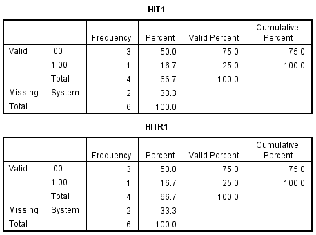
Suppose you wanted to create a dummy variable from trial1 with a cutpoint of two. We can use the if command to create the variable hit1. The same is true for creating hirt1 from trialr1.
IF trial1 > two hit1 = 1. IF trial1 <= two hit1 = 0. IF trialr1 > two hirt1 = 1. IF trialr1 <= 2 hirt1 = 0. VARIABLE LABELS hit1 "Tran T1 User Miss" hirt1 "Tran T1 Sys Miss". FREQ /VAR= hit1 hirt1.
The frequencies shows the outcome of these transformations as they touch on the missing values. Both system-missing and user-defined missing values result in correct classification.
Now, suppose you wanted to create a dummy variable from trial1 in combination with trial2 with a cutpoint of two for each. We can apply the if command to create the variable hit12. The same is true for creating hirt12 from trialr1 and trialr2.
IF trial1 > 2 and trial2>two hit12 = 1. IF non(trial1 > 2 and trial2>2) hit12 = 0. VARIABLE LABELS hit12 "Tran T1 AND T2". FREQ /VAR= hit12 . List /VAR = trial1 trial2 hit12.
The frequencies and listing shows the consequence of these transformations as they touch on the missing values. Both arrangement-missing and user-defined missing values result in the same output, and then but the output for user-defined missing values will be shown.
TRIAL1 TRIAL2 HIT12 ane.fifty 1.40 .00 1.l -nine.00 .00 -9.00 two.00 .00 -9.00 -ix.00 . 2.10 2.thirty ane.00 1.80 ii.00 .00
At that place is but i missing value in the created variable hit12, merely we know that there are at to the lowest degree 2 missing values for trial1 alone. If SPSS tin can resolve the logic based on a unmarried variable, then it will. Since not(trial1 > 2 and trial2>ii) is truthful if either of the atmospheric condition is false, this can be resolved. This is the result that most people would prefer.
If you prefer to have the consequence missing if either of the component variables are missing then that can be accomplished past adding the post-obit if command. As is shown by the results of the frequencies and list commands.
IF MISSING(trial1) OR MISSING(trial2) hit12 = $SYSMIS. FREQ /VAR= hit12 . LIST /VAR = trial1 trial2 hit12.
Annotation that the missing function is evaluated as true if the variable in the argument contains any kind of missing value. If you lot are exclusively concerned with system-missing values you may want to use the sysmis function. Consider the following results. Any missing value for i of the component variables results in a missing for hit12 .
TRIAL1 TRIAL2 HIT12 ane.50 1.40 .00 one.50 -9.00 . -nine.00 2.00 . -9.00 -ix.00 . 2.10 2.30 1.00 1.80 ii.00 .00
Using RECODE
The recode control can be used to accomplish the dummy coding task discussed at the outset of the department. In one case again, suppose yous wanted to create a dummy variable from trial1 with a cutpoint of 2. Nosotros can use the recode control to create the variable hit1. The same is truthful for creating hirt1 from trialr1. Yet, this command functions differently with respect to arrangement-missing and user-defined missing values.
RECODE trial1 (LO THRU two=0) (ii THRU HI=one) INTO hi2t1. RECODE trialr1 (LO THRU 2=0) (two THRU Howdy=i) INTO hi2rt1. VARIABLE LABELS hi2t1 "Tran T1 User Miss" hi2rt1 "Tran T1 Sys Miss". FREQ /VAR= hi2t1 hi2rt1.
The frequencies shows the result of these transformations every bit they affect the missing values. The answer is correct with respect to system-missing values and incorrect with respect to user-missing values. The user-defined missing values are classified according to their value, as if they were not missing.
At present we can examine recode with the else keyword. This affects both system-missing and user-defined missing values the aforementioned, but unfortunately neither are right. The else keyword will include both types of missing values, and mis-classify them.
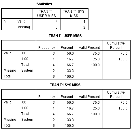
RECODE trial1 (LO THRU 2=0) (ELSE=1) INTO hi3t1. RECODE trialr1 (LO THRU two=0) (ELSE=1) INTO hi3rt1. VARIABLE LABELS hi3t1 "Tran T1 User Miss" hi3rt1 "Tran T1 Sys Miss". FREQ /VAR= hi3t1 hi3rt1.
The frequencies result follows.
If we add the (missing=sysmis) to the recode the trouble is alleviated for system-missing , just non for user-divers missing values.
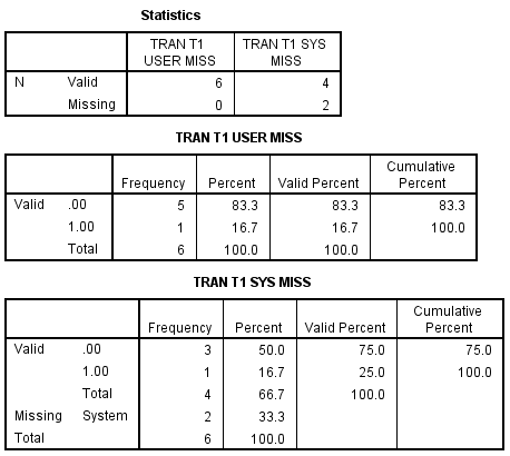
RECODE trial1 (LO THRU 2=0) (MISSING=SYSMIS) (ELSE=1) INTO hi4t1. RECODE trialr1 (LO THRU 2=0) (MISSING=SYSMIS) (ELSE=1) INTO hi4rt1. VARIABLE LABELS hi4t1 "Tran T1 User Miss" hi4rt1 "Tran T1 Sys Miss". FREQ /VAR= hi4t1 hi4rt1.
The frequencies result follows.

Changing the gild of (missing=sysmis) and (lo thru two=0) alleviates the trouble for user-divers missing too.
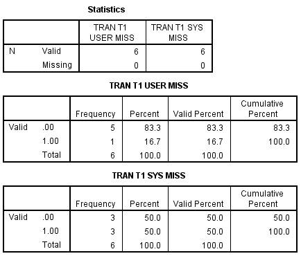
RECODE trial1 (MISSING=SYSMIS) (LO THRU 2=0) (ELSE=1) INTO hi5t1. RECODE trialr1 (MISSING=SYSMIS) (LO THRU 2=0) (ELSE=1) INTO hi5rt1. VARIABLE LABELS hi5t1 "Tran T1 User Miss" hi5rt1 "Tran T1 Sys Miss". FREQ /VAR= hi5t1 hi5rt1.
The frequencies issue follows.
8. Issues to await out for
- When creating or recoding variables, it is always good practice to examination the resulting variables, especially for missing values.
- The type of missing value can make a deviation in recode results, and in most cases sytem missing values are more likely to yield the correct results.
- Be enlightened how the utilize of and and or work with the if control, equally the expression is evaluated, and if a logical decision tin be made, it will be made. This happens fifty-fifty though one or more of the component variables may be missing.
9. For more than information
- Come across Subsetting information in SPSS for information well-nigh subsetting data with variables that are missing.
- For more information about missing values, see the SPSS Command Syntax Reference Guide .
rodriguezhantimpok.blogspot.com
Source: https://stats.oarc.ucla.edu/spss/modules/missing-data/
0 Response to "Read Multiple Variables Create New Variable if Not Blank Spss"
Post a Comment